How ClickHouse saved our data

The Mux Data platform is used by some of the biggest broadcasters to monitor the video streaming experience of their end users. Think of it like Google Analytics or New Relic for video playback. It's an essential tool that our customers rely on to make sure they are delivering smooth video.

Mux Data processes billions of video views every month and gives users a way to query views in real-time as data is being collected. Over the past few months we have been transitioning the storage of video views from a sharded Postgres database to a ClickHouse cluster, with great results. In this post, I'll share our legacy architecture, the new ClickHouse architecture, the performance improvements, and finally some tips on how we're leveraging the best parts of ClickHouse to build a better and more robust data product for our customers.

What's in a View?

Every video view consists of dimensions (properties of that view) and metrics (measurements of what happened during the view). In total we record around 100 each of dimensions and metrics, meaning the resulting schema has almost 200 columns. This data is stored for up to 90 days.

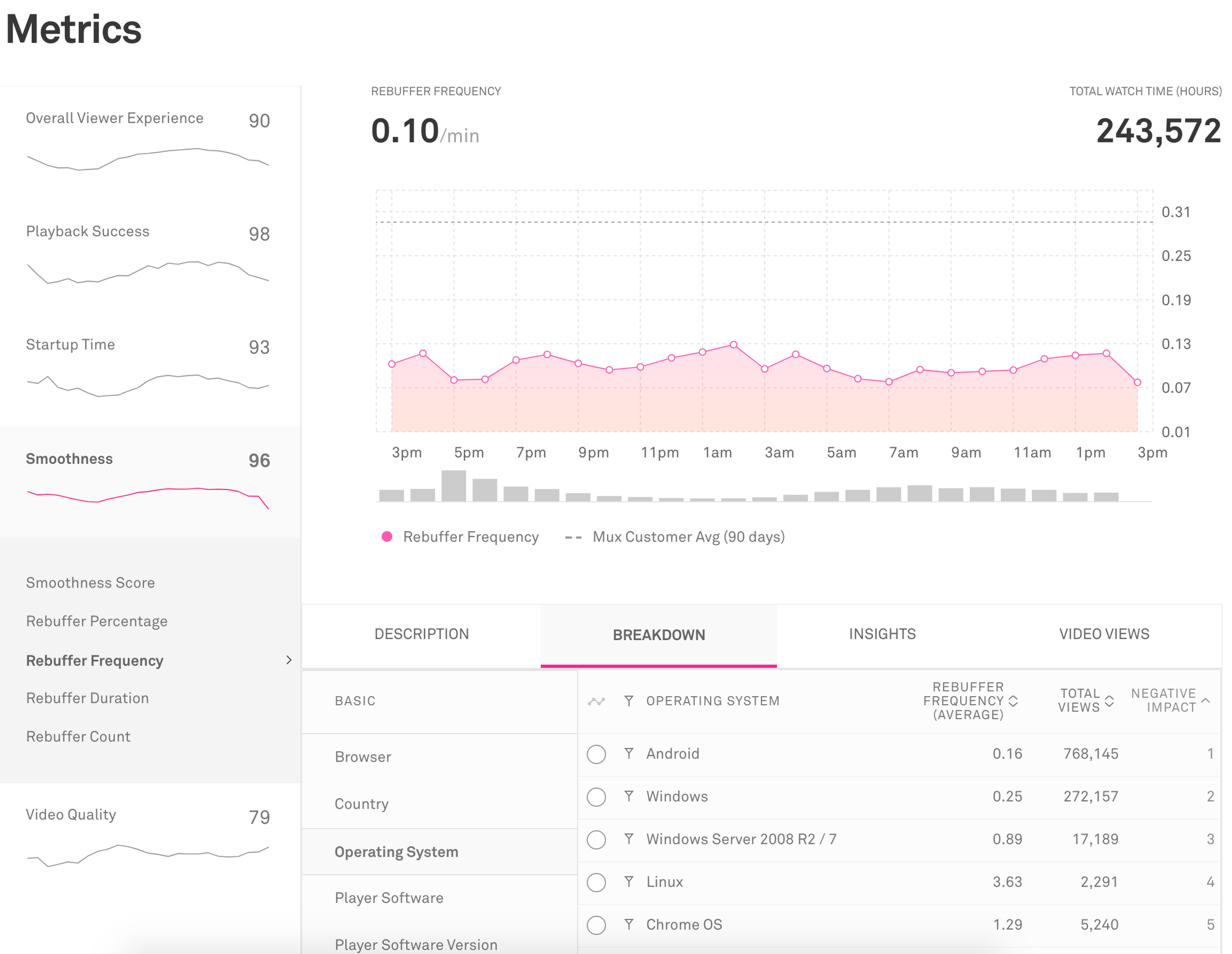
One of the main uses of Mux Data is to view a specific metric aggregated over both time and a dimension. For example, customers can see the rebuffering frequency of their viewers over the past 24 hours, as well as broken down by operating system.

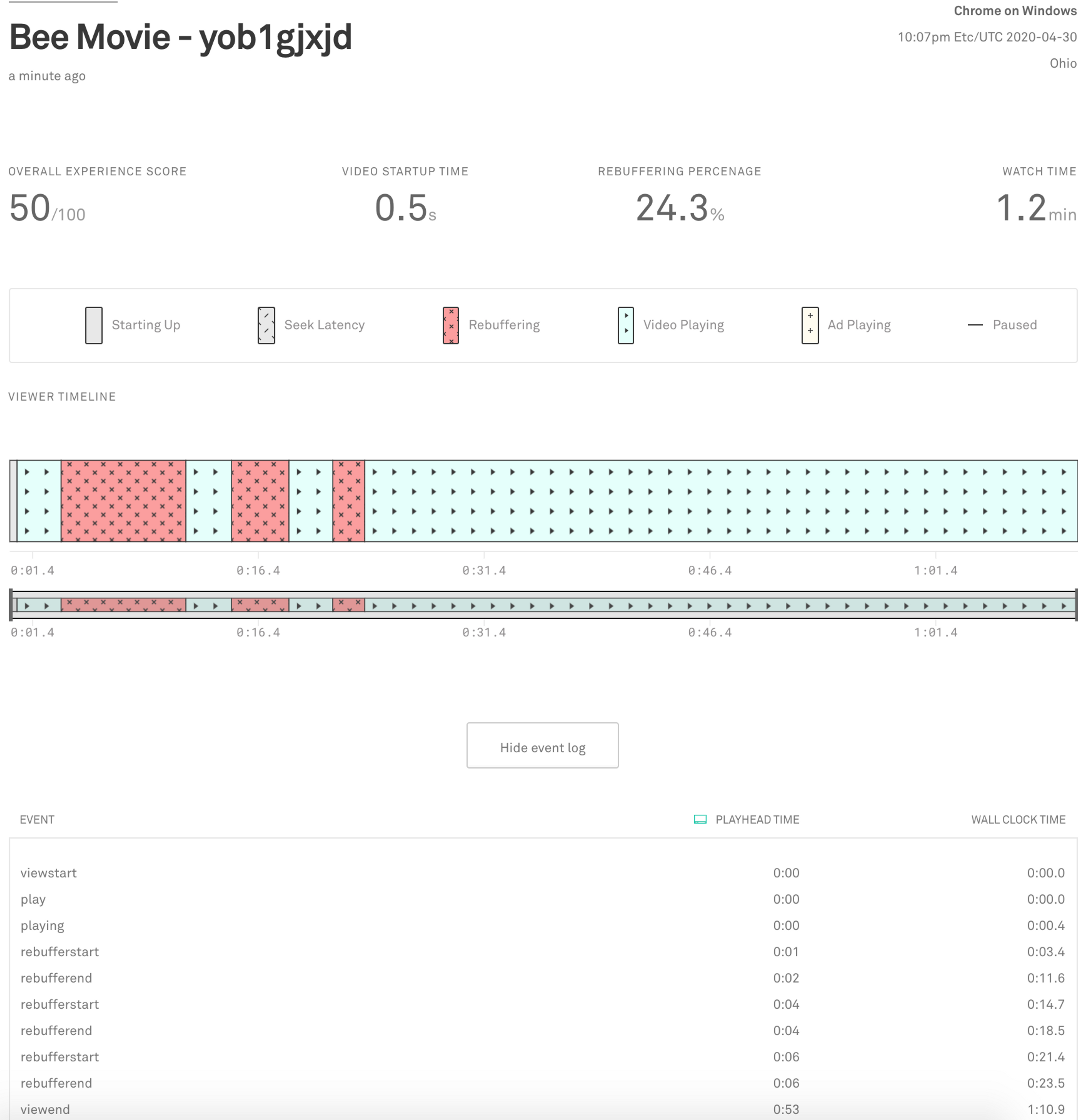
Customers can also drill down into a single video view to see the exact sequence of events, as shown below.

From these two views, we can see that views must be both individually queryable, and grouped by arbitrary dimensions and time buckets. Let's dive in to how we first achieved this.

Before ClickHouse

Our original architecture consisted of multiple, sharded, Postgres databases, as well as Airflow workers that performed aggregation. The three sharded Postgres databases were

1. views: stored all columns of a view, for detail view queries and long-running metrics aggregation
2. slim_views: stored a subset of columns, for sub-hour metrics queries
3. aggregates: stored aggregated values, for hourly- and daily- metrics queries

Airflow jobs would then run against the views database each hour to populate aggregates with metrics in hourly buckets. Daily Airflow jobs would also aggregate hourly buckets into daily buckets. Each database was sharded by customer in order to minimize the impact large queries from one customer may have on others.

The slim_views database stored a full copy of the data, but only included metric and filter columns (around half of all columns). This greatly improved the performance of metrics queries for time ranges that had not yet been aggregated (i.e. the last 45 minutes).

The Woes of Aggregation

In the legacy architecture, aggregation was necessary to achieve acceptable performance on any query spanning more than a few hours. This is because Postgres would have to scan over all of the rows matching that customer and time-frame, applying any filters and computing the average or quantile in question. While aggregation kept the system running, it came with a few big limitations.

Limited Filtering

When performing aggregation, any possible filter combination we want to support must be queried for and stored. The cardinality of the aggregates is then exponential in the number of filters we wish to support. For example, suppose we want to support filtering on video_title, operating_system and country. The number of aggregates computed and stored will be (# video titles) * (# operating systems) * (# countries). With some dimensions having hundreds of thousands of values, the size of the aggregates gets out of hand very quickly. For this reason, we had to limit customers to a maximum of three filters.

Operationally Fragile

Computing all of these aggregates was no small task. Airflow jobs were constantly querying slim_views to create hourly aggregates. If too many jobs that landed on the same Postgres shard happened to run at the same time, the cluster could grind to a halt. This required manually stopping all of the other jobs and babysitting them one-at-a-time until they all completed. During these incidents, aggregation would fall behind and raw data from slim_views would have to be used for larger portions of the time-frame being queried for. This could create a negative feedback loop and potentially downtime while aggregation caught back up to the last hour.

Difficult to Change

The logic for combining data across daily-, hourly-, and row-level aggregates was encoded in around twelve-thousand lines of store procedures. These stored procs took care of everything from sharding to filtering to falling back to finer-granularity aggregates. In order to make a simple change like adding a new dimension, which would normally be a single ALTER TABLE statement, the stored procs had to be reasoned about and carefully edited to be backwards compatible. We were all but terrified of making changes to these stored procs.

When revisiting this architecture, it was clear to us that we should do everything in our power to avoid the need for aggregation, and that's exactly what we achieved by switching to ClickHouse.

Bring in the ClickHouse

You might be wondering "what on earth is a ClickHouse?" ClickHouse is an open-source analytics database designed at Yandex, and it's really fast. ClickHouse achieves speed in two major ways

1. Column-oriented compression. In ClickHouse, data is separated, compressed, and stored by column. Since consecutive values in the same column are likely to have repeating patterns, this compresses extremely well compared to row-based storage systems.
2. Sparse indices. When a data part is written to disk, the rows in that part are sorted by primary key, and every n-th row's primary key is written to a sparse index, along with the offset in the part of that row. By default n = 8192, so the index is thousands of times smaller than the primary key column and can be kept in memory. The ClickHouse documentation has a great explanation of sparse indices and how they are searched and maintained.

With all of this in mind, we started by keeping the architecture as simple as possible: just dump all of the data into one table called views. No Airflow. No aggregation. No stored procedures. Any bucketing logic would be written in the SQL queries at read-time and computed on the fly.

To our surprise, this worked extremely well. We could query over large time-frames of data, specifying an arbitrary number of filters. ClickHouse's columnar storage is a massive benefit when the data has very wide rows, like our views schema. Even though there are 200 columns, only the columns corresponding to the filters being used and the metrics being aggregated have to be read from disk.

Here's a small slice of our table schema:

CREATE TABLE views (
    view_id UUID,
    customer_id UUID,
    user_id UUID,
    view_time DateTime,
    ...
    rebuffer_count: UInt64,
    --- other metrics
 
    operating_system: Nullable(String),
    --- other filter dimensions

)
PARTITION BY toYYYYMMDD(view_time)
ORDER BY (customer_id, view_time, view_id)

By the Numbers

Our goal when we set out to re-implement our metrics backend was for the p95 latency of all front-page queries to be under one second. This includes the time-series chart, breakdowns, and sparklines on the sidebar. Every filter, dimension, or metric selection blocks on re-execution of these queries. With a product meant for exploring data, optimizing these queries was pivotal to giving an interactive feel.

During development we found that ClickHouse was so efficient that we started measuring p99 latency of queries instead of p95, with the goal of all front-page queries being as close to under one second as possible. To test performance, we mirrored all production queries to both Postgres and ClickHouse, but validated and threw away the ClickHouse response. In this way, we measured performance differences between individual queries to catch any potential regressions. Below is a chart of two weeks of this mirroring over all of our production load.

A few things to note:

1. ClickHouse out-performed our sharded Postgres setup by at least 2x on all queries, even while doing all aggregation on-the-fly.
2. Complex queries like "Insights" would frequently timeout client-side when sent to Postgres, but ClickHouse finishes the vast majority in under 5 seconds.
3. ClickHouse is still faster than the sharded Postgres setup at retrieving a single row, despite being column-oriented and using sparse indices. I'll describe how we optimized this query in a moment.

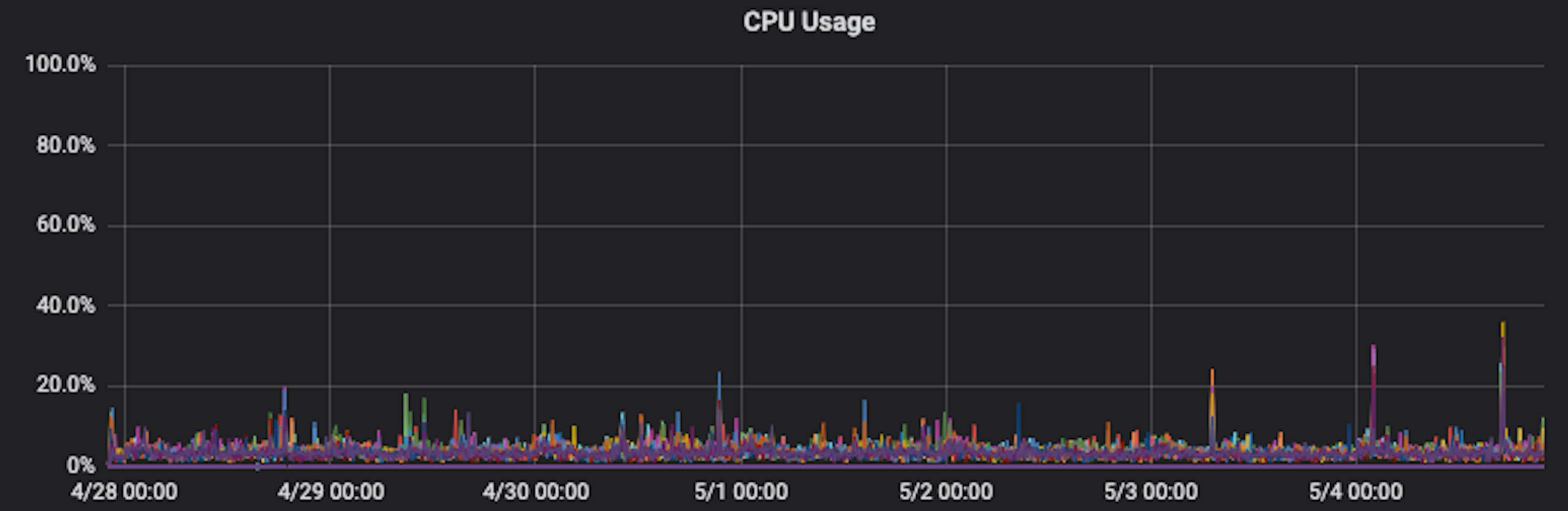
Needless to say, we were extremely happy with the performance of the new system. In my experience, it is most tractable to architect systems for ~10x increase in scale. ClickHouse very much accomplished that for us, as illustrated by the steady-state CPU utilization of the cluster:

Making it Work

There are many blog posts-worth of knowledge we've gained over the course of this migration, and I'll share a few of the notable learnings here.

Querying by ID

The columnar and sparse index aspects of ClickHouse make querying for a single row of data less efficient, especially when querying by something that is not in the primary key (which determines the sort order of the sparse index).

In our case, we had to support both querying by a single view id, as well as listing all views for a given user id. However, our primary key is of the form (customer_id, view_time), so a naive query for user id or view id for a given customer would have to scan all view_times for that id.

Early tests showed that the naive query would be prohibitively expensive, taking a few seconds on average. Luckily I stumbled upon this great blog post by Percona that explained how to use ClickHouse materialized views as indices, although I wouldn't recommend using ClickHouse as your "Main Operational Database" just yet.

The basic idea is to create another table that will serve as your index, with a primary key equal to the field you'd like to index on. Alongside the indexed column, you also store the primary key of that row in the original table. To look up a single row, first search the materialized index by the id to retrieve the primary key of that row in the original table. Then search the original table using that primary key prefix.

For example, in our case the main table's primary key is (customer_id, view_time). To create an index on user_id, we create a user_id_index table with primary key (customer_id, user_id), and an addition column view_time. The materialized view for the user_id_index table stores the customer_id, user_id, and view_time of every view written to the main views table. Then to search for all views for a specific (customer_id, user_id), we search user_id_index for all corresponding view_times, then query the views table using those view_times. This can all be wrapped up into a single query like

SELECT * FROM video_views
WHERE
    view_time IN (
        SELECT view_time FROM user_id_index
        WHERE customer_id=0 AND user_id='kevin'
    )
    AND customer_id=0 AND user_id='kevin'

Note that any additional WHERE clauses have to be repeated in both the index query and the main table query since view_time is not a unique value.

Using materialized indices was extremely effective, bringing our average single-row query latency down from a few seconds to just 75ms.

"Mutating" Data without SQL UPDATE

Another relatively simple operation in Postgres is updating a row when data has changed. In our system, this is required when a view resumes. An example of this would be a user pausing a video, coming back five minutes later, and watching the rest. We don't want to delay the data from the start of this view, so we store the beginning of the view up until the pause in the database and then UPDATE the row if a resume occurs.

However, ClickHouse does not have the same notion of a SQL UPDATE statement. Data parts are treated as immutable groups of rows (split up by each column). In order to change a single value, ClickHouse has to rewrite that entire data part and the corresponding sparse index offsets. Data parts can easily be gigabytes of data, so doing this for every view resume would be prohibitively expensive.

Instead, ClickHouse implements a few table engines that allow updates to rows to eventually be merged into one row. We chose the CollapsingMergeTree, in which every row is assigned a Sign of 1 or -1 on insert. When data parts are merged, rows with the same primary key and opposite Sign cancel each other out and are omitted.

We modified our rollup/insert pipeline to store the last state written to ClickHouse when a view is resumed. When the updated view is eventually written to ClickHouse, the old state is written as well with a Sign of -1.

Before both positive and negative rows of a view are merged into the same data part, they will co-exist in ClickHouse. This means that queries will be double-counting views that resume unless the queries are adjusted, which is made possible using the Sign column. To compute a COUNT(), we instead compute SUM(Sign). Similarly, AVG(metric) is instead computed as SUM(metric * Sign) / SUM(Sign). While this added some complexity to our query layer, it made view resumes just as performant as normal inserts.

Looking Ahead

Transitioning our long-term analytics storage to ClickHouse proved to be extremely worthwhile in the end. It really does feel like a database designed for the 21st century, with support for modern formats and integrations like Protobuf and Kafka.

We have productionized ClickHouse inside of a Kubernetes cluster, complete with sharding and replication to eliminate any single point of failure. I look forward to sharing more of the operations and deployment side our experience with you in the future.

As next steps, we are always looking for ways to take further advantage of ClickHouse, including optimizing queries with Materialized Views, replacing the rollup process with AggregatingMergeTrees, and architecting an efficient real-time query layer.

If these types of problems interest you, definitely check out our open positions at mux.com/jobs! Another great way to get involved is to attend the ClickHouse meetups organized by Robert Hodges of Altinity (a wealth of ClickHouse knowledge).

I hope you enjoyed the post! Be on the lookout for more ClickHouse stories, tips, and tricks from us in the future as we continue to bring Mux Data to the next level.